


How To Create Procedural Landscapes in Blender 4.3
Create "Heightfields", Layer Noise, & Simulate Fake Erosion with Geometry Nodes


When we think of proceduralism, we often think about buildings springing up from simple base shapes or forests emerging from a collection of parameterized trees, plants, and other foliage. However, in recent years the DCCs that we all work with have gotten more capable. Truly procedural worlds now consist of generated landscapes and terrain based on intricately crafted logic. As computers have become capable of calculating complex math equations at faster speeds, so too have those benefits been felt across the 3D world. After all, at the end of the day digital 3D art is just a bunch of math creating the mesmerizing worlds we see.
Blender is a recent newcomer to the procedural world, with it’s own Geometry Nodes toolset providing users with a small, but growing, set of tools to work with. As we’ve discussed in previous articles, Geometry Nodes is exceptionally powerful, but it still leaves much to be desired when compared to tools like Unreal Engine or Houdini. Yet, Geometry Nodes are still capable of doing some very intricate work. Over the past two weeks I’ve been investigating its application on procedural terrain, and I’ve found some fairly surprising results.
In this guide we’ll be covering:
Procedural Terrain Basics
Layering Noise For Finer Detail
Implementing “Fake” Erosion Simulations
With that said, let’s move onto today’s guide. (If this article is cut-off in your email, you can view the rest in your browser or in the Substack App.)
3D Terrain Heightfields
Creating a 3D environment entails a lot, but the key element that holds everything together (literally) is the terrain that everything is placed on. If you load into an open world video game or look into the backgrounds of cinematics, it’s more than likely that you’re looking at a 3D heightfield. While the ground we stand on IRL is completely solid, heightfields are actually just planes deformed by heightmaps or height values. Technically a heightfield is any geometry that’s manipulated by some procedural process (namely erosion), while any flat geometry can be considered a piece of terrain.
For our purposes, Blender doesn’t natively support heightfield manipulation like Unreal Engine or Houdini does. However, at the end of the day those DCCs are just taking a plain and manipulating the positions of the vertices in specific ways. So technically there isn’t anything stopping us from using Geometry Nodes to do what those DCCs are doing. We just don’t have the optimizations to run everything as smoothly as they do.
Basic Node Setup
To create a heightfield, all you really need is a grid with the desired number of subdivisions and a noise source. Most games that generate terrain at or in runtime use Perlin Noise, a specific type of noise which (fortunately for us) Blender uses as it’s basic Noise function.

The picture above shows the barest setup you can use to manipulate the height of the grid with the noise of a Noise Texture node. Note that because the Offset socket on the Set Position node is a diamond field socket, the value that’s connect to it it being evaluated per element (vertex in this case).
We’re able to apply the noise because Geometry Nodes is matching the 2D position of the Noise Texture to the 3D position of the vertices. Then, the factor of the Noise Texture is transferred to the Z axis value of the vertices. If we make the size of our Grid larger, the scale of the noise stays the same but we see more of the noise because the position of each vertex now corresponds to a different noise factor value.

Before we move onto the next step, we can also re-center the heightfield at the origin by using this node setup:

Layer Noise
Using one Noise Texture node to manipulate our heightfield works, but it doesn’t look very realistic. If we were using Houdini to create our heightfield, we might use Erosion simulations to help use get a more realistic shape. However, erosion simulations take time and aren’t capable of being procedurally generated since they rely on recreating how fluids interact with the terrain. It’s also not possible to use erosion simulations inside of Blender, at least not in the base software.
Instead, we’ll be utilizing multiple layers of noise to help us get a more realistic shape, and in the next section we’ll be altering the way we apply these noise layers to get to our final heightfield shape. As we go along we’ll also be exposing more parameters to be modified from the panel modifier as well, giving us better control over the shape of the heightfield without requiring us to be in the node graph.
Repeated Random Noise Node Setup
To apply multiple layers of noise to out heightfield, we’re going to be utilizing a Repeat Zone. We’ll be going over the individual components in just a second, but here is the full node setup.

Each iteration (or loop) of the Repeat Zone will layer a new layer of noise with a random rotation over-top of the previous geometry. We pass the generate noise factor value (in the form of a vector) out the end of the Repeat Zone so that we can add it on top of the noise created in future iterations.
We connect the Grid node’s Mesh output socket to the starting Repeat Zone node, and then the Geometry socket of the ending Repeat Zone node to the Recenter Noise node setup we showed in the last section.
To change the noise on each iteration, we use one node setup to first alter the physical properties of the noise, and a second setup to change the orientation.
Noise Properties

We can use a Map Range node to create the intervals of change for the noise properties by plugging the Iteration output socket of the starting Repeat Zone node into the Value input socket on the Map Range node. Then we make sure that the From Max input socket on the Map Range node is equivalent to the Iterations input socket on the Repeat Zone starting node by either setting a constant Integer node, or by connecting both to an empty socket on the Group Input node. Doing the latter allows you to control both of these sockets with one value on the modifier tab instead of in the node graph.
Then, we take the Result output socket of the Map Range node and connect it to the Value input socket of a Float Curve node. Invert the control points on the curve graph area, and set a curve profile to alter the strength of the node.
Finally, create two Math nodes set to Multiply and connect the Value output socket of the Float Curve node to the first Value input sockets on both Multiply nodes. The first Multiply node will control the Scale socket of the Noise Texture, while the second will control the Detail socket. If you’d like, you can also connect the Value output socket of the Float Curve node to the Roughness input socket on the Noise Texture as well.
Noise Orientation

The Vector input socket on the Noise Texture node controls the position of the noise in it’s relative space. In my node setup, I have a Random Value node (set to Integer) that feeds into a Vector Rotate node to randomly rotate the noise. The Seed input socket on the Random Value node is connected to an empty socket on the Group Input node, allowing me to change the random value at will.
I also have a Vector Math node set to Add that allows me to specify an offset value to move the noise by. Again, this allows me to control the position of the noise, which will move how the noise affects the height of the heightfield.
There are many ways to use the Vector input socket on the various Texture nodes, so I would highly recommend experimenting with your own setups.
“Fake” Erosion Simulations
I mentioned in the last section that Blender doesn’t natively support erosion simulations. While this is true, we have ways of “faking” the effects of erosion by using mathematical formulas to our advantage. The technique that we’ll use is called a Finite Derivative Approximation1, but it’s nowhere near as complicated as it sounds.
The technique boils down to calculating the slope of our noise values at every point, and using it to “erode” (read: decrease) the height based on how steep the slope is. Points that have a high slope value will erode faster, while points with a low slope value won’t. Before you look over the node setups that I’m about to show, take a moment to go over the steps that are actually happening. The nodes will look intimidating, but the process isn’t that complex.
Finite Derivative Approximation in Geometry Nodes
The process goes as follows:
Create an initial layer of noise.
Calculate the height of an Active Point, one point to the Active Point’s right, and one point in front of the Active Point.
Find the Gradient (Read: 2D Slope) of the Active Point by finding the Derivative (Read: 1D Slope) of both the X and Y axes.
Calculate the Magnitude of the Gradient (Read: How strong the 2D slope is).
Decrease the noise layer by the Magnitude.
Pass the Gradient Vector Field (Read: The direction the slope ascends in) to the end of the Repeat Zone.
Add the Gradient Vector Field values to the Gradient Vector Field values of the next noise layer before finding the Magnitude of the next layer.
Repeat for every layer of noise.
Starting Nodes (Step 1)
For clarity’s sake, I’ve condensed the nodes from the first two sections into node groups. They are labeled by their purpose, and their outputs are also labeled to show what values you need to output from those node groups. Here’s a picture of the nodes at the start of the Repeat Zone. You don’t need to plug every parameter into the Group Input node, however I find it easier to adjust from the side panel rather than moving in and out of node groups.

Calculating Finite Derivative Approximation (Steps 2-4, 6-7)

We take our HeightValue attribute (noise values) and perform all of the calculations on them. At the end of this, we store the Gradient Field Vector (Slope Direction) and the Gradient Magnitude (Slope Steepness) in point attributes to reference them later on.
Calculating Noise Height Values (Step 2)

Our Active Point is determined by the Index node. We then need two more points, one to the Right/Left and one in Front of/Behind the Active Point. We can use the Resolution parameter (how many divisions our grid has) to ensure we aren’t selecting a Right/Left point that doesn’t exist, and use the Increment parameter (how many points ahead we’re looking) to do the same for the In Front/Behind point. A Switch node determines whether to select a point to the Right or Left point, as well as a In Front or Behind point. Then we sample the HeightValue attribute at the selected points using a Sample Index node.
Calculating Derivatives (Step 3, 7)

The Gradient Vector Field is the combination of the X and Y Derivatives. Calculating a Derivative (as far as we’re concerned) is calculating the Slope (Rise/Run) between two points at a fixed distance.
Calculating Magnitude (Step 4)

The Magnitude is the strength of the Gradient Vector Field. It also happens to be the exact same equation as Pythagoras’ theorem.
Applying Magnitude To Noise Height (Step 5)

We use the Magnitude to “erode” the current layer’s noise value. These are just math nodes that decrease the noise value according to a specific function. You can apply any math formula here to generate a different type of “erosion”.
End Nodes (Step 6, 8)
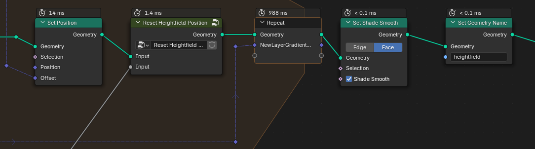
The eroded Noise value is applied to the Grid, and the re-centered using the node setup from the first section. The Gradient Vector Field is passed on to the next iteration.
Top Level Node Group Overview

Outcome

In this guide we went over using noise to drive procedural terrain creation with Geometry Nodes. Iterating over three methods of doing so has given us a fine amount of control over the look of our terrain, however there is still more that could be done. For instance, we could use multiple setups with different profiles to blend between different terrain types. Or we could feather the height profile at the edges of the mesh so that we can lay it among other non-procedurally generated terrain. There is still a lot that can be done, so be sure to play around with these setups and see what you can make!
- Adam