

Manipulate Data In Geometry Nodes
Working With Attributes, Fields, & Instances in Blender 4.3


Once you’re familiar with creating and interacting with Geometry Node Groups, it’s time to look at what’s actually happening.
As I’ve mentioned before, 3D geometry is just a collection of vertices that are joined together to form edges and faces. Every vertex is a set of three coordinates in 3D space. We can add in more data for more utility, like what faces they’re apart of, and then add in data on top of those faces as well.
Geometry Nodes allows us to access all of these values and manipulate them without needing to write any code. All we need to do is connect the nodes, assign the attributes, and guide the process.
In this article, we’ll be looking at all of the big ways to work with Attributes, Fields, and Instances, along with some clever methods for achieving some not-so-obvious tricks within Blender’s Geometry Nodes.
Quick Aside:
In last week’s article I made the mistake of referring to all node Sockets as Fields. Fields are a special type of node-and-socket combination, while Sockets are just the physical connector for every node. I’ll explain more later on in this article, but I just wanted to highlight the mistake and let y’all know that I’ve corrected the mistakes in last week’s article.
Attributes
We’ve gone over Nodes, Sockets, and Connections last week, so we’ll pick up where we left off.
All nodes accept and pass values through Sockets. Sockets on the left side of the node input data, while Sockets on the right side output data. If you hover your mouse over a Socket, you’ll be able to see what is being passed in or out.
However, these “values” are more important than just being numbers or strings. They pass Attribute data, or information about the geometry it originates from. Index (ID), Position (Location), and Normals, are all Attributes and have corresponding nodes that can be accessed in a node group.
The Inspector sheet can be used to view Attributes in their different Domains. An Attribute Domains refer to what the Attribute is stored in, and can be anything from Vertices, Edges, Faces, UVs, Volumes, Curves, or even Instances.
Each Attribute has a specific data type, meaning you can’t pass different data types into each other. The full list is too long for one article, so I’ll link to the Blender Documentation where the full list is explained.
Fields

We can access Attributes through special nodes called Field nodes. They are marked with Diamond sockets rather than Circle sockets. Some nodes might come with both types of sockets, which means that they can work with Field values, but aren’t always required.
A Field node doesn't directly give a value; it instead tells the node where to get that value. For example, an Index Field node will tell the connected node to look at the incoming geometry to find the Index (ID) of each vertex.
Fields might contain a Dot contained inside the Diamond socket. This shows what type of data is being brought in. If a Field socket has a Dot, it means that the same value is being applied across all elements of the geometry. While no Dot means that the data is unique to the element of the geometry it's being applied to.
Field data is evaluated backwards from the connecting sockets. This means that if you connect the same Field node to two different geometries, you might get two different values depending on what data is attached to those geometries.
If we want to capture any values that results from a Field node, we can use the Capture Attribute node to store that value. That way the value is able to be referenced at any time by connecting the output Field node of the Capture Attribute node to the desired downstream node.
Instances
A final related concept is Instancing. The easiest way to conceptualize an Instance is by thinking of it as a reference to an existing piece of geometry. Usually Instancing is done over points or other individual elements, so when the output of the node group is displayed in the viewport you’ll see a copy of the referenced geometry at every point you’re Instancing on. However, the Instanced geometry doesn’t technically exist.
The benefits of Instancing geometry lies in optimization. Instead of actually placing down down hundreds of objects, we can make one and Instance it over a group of points. This can also be detrimental if not thought out though. Applying a Subdivision Surface node before Instancing means it's only being applied to one geometry. Whereas if it's applied after Instancing, it's being applied to all of the Instances.
Instances can also be sub-nested into more Instances. Blender only supports 8 iterations of instancing in the viewport though, so make sure that if you continue to instance that you realize your geometry at some point. To realize the Instanced geometry, we have to use a Realize Instances node to make it real.

Examples
Change Scale Based On Curve Profile
We can use an Index node and a Float Curve node to drive the scale of Instanced geometry. The Index node tracks the placement of each point we Instance on, while the Float Curve node determines the profile of the scaling factor.
Setup
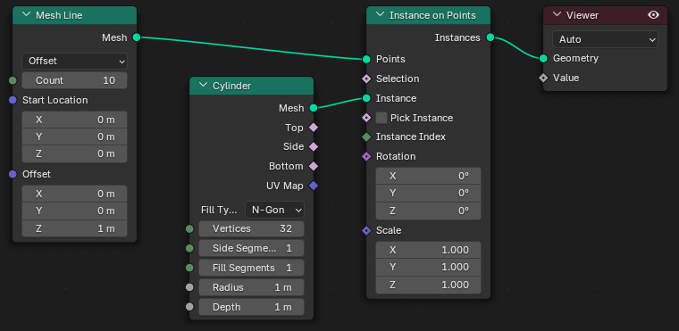
Place a Mesh Line node, a Cylinder node, and an Instance on Points node. Connect the Mesh Line nodes Mesh output socket to the Points input socket on the Instance on Points node. Connect the Cylinder nodes Mesh output socket to the Instance input socket on the Instance on Points node.
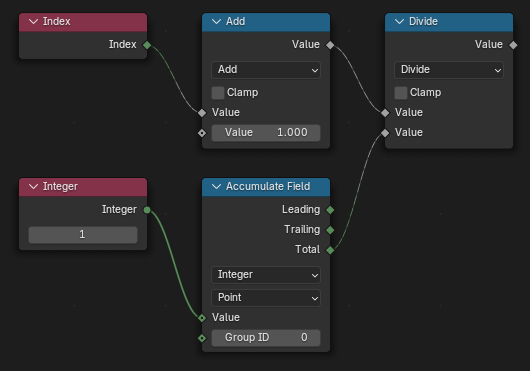
Place an Index node, Two Math nodes (one set to Add, the other to Divide), an Integer Constant node, and an Accumulate Field node.

Connect the Index node output to the Add node (set the other value to 1), and then the Add nodes Value output socket to the first Value input socket on the Divide node.
Set the Integer node to a value of 1 and connect its output socket to the Value input socket on the Accumulate Field node. Make sure the Accumulate Field node is set to Integer and Point values in the drop down menus. Connect the Total output socket to the bottom Value input socket of the Divide node.
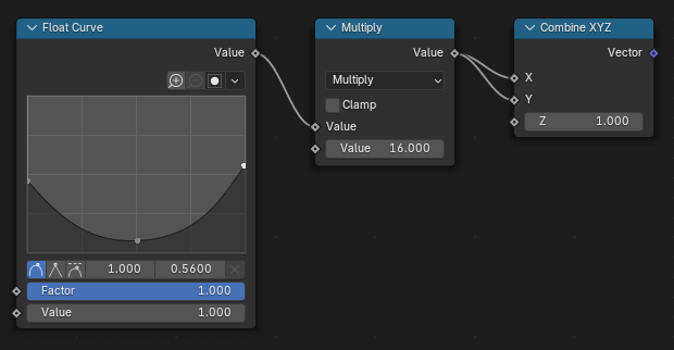
Place down a Float Curve node, a Math node (set to Multiply), and a Combine XYZ node. Connect the Float Curve Value output socket to the first Value input socket of the Multiply node. Then connect the Multiply Value output socket to both the X and Y input sockets on the Combine XYZ node.
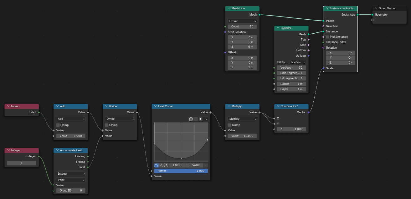
Finally, connect the Value output socket of the Divide node to the Value input socket on the Float Curve node. Connect the Vector output socket of the Combine XYZ node into the Scale input socket on the Instance on Points node.


Result
The Float Curve node allows us to control the X and Y scale of the Cylinders that we Instance. Since we’re Instancing on a Mesh Line, we can use the Index Field to calculate where each Instanced Cylinder should be placed along the Float Curve profile.
Extrude By Proximity
Geometry outside the Node Group also have Fields that we can access and manipulate. By bringing in such geometry, we can influence the behaviour of the Node Group.
Steps
(Outside of the Node Group) Place an object in the scene to act as the driver object.
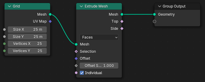
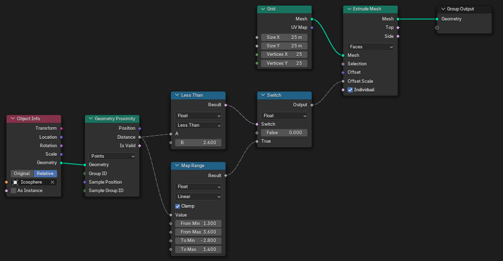
(Inside the Node Group) Place a Grid node and an Extrude Mesh node. Connect the Mesh output socket of the Grid to the Mesh input socket of the Extrude Mesh node. Make sure the Grid node has enough Vertices and is big enough to be affected by the driver object.

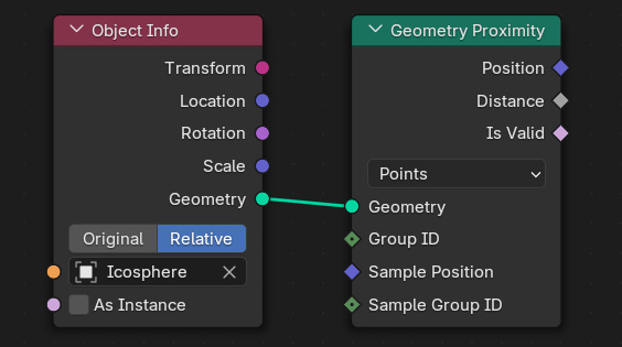
Drag the driver object from the Outliner into the Node Editor. Place down a Geometry Proximity node. Connect the Geometry output socket of the driver’s Object Info node into the Geometry input socket of the Geometry Proximity node. Make sure the driver’s Object Info node is set to Relative.

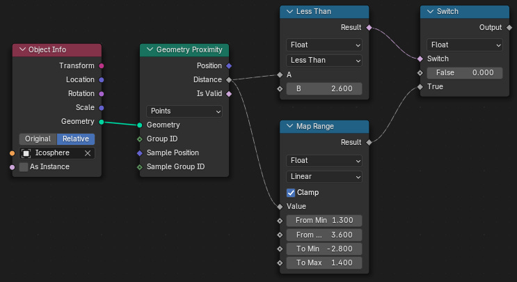
Place down a Map Range node, a Compare node (set to either Less Than or Greater Than), and a Switch node (set to Float).
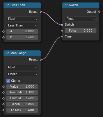
Connect the Distance output socket of the Geometry Proximity node into both the Value input socket of the Map Range node and the A input socket of the Compare node.
Connect the Result output socket of the Compare node to the Switch input socket of the Switch node. Leave the False input socket at 0, and connect the Result output socket of the Map Range node to the True input socket of the Switch node.

Connect the Output value socket of the Switch node to the Offset Scale input socket of the Extrude Mesh node.

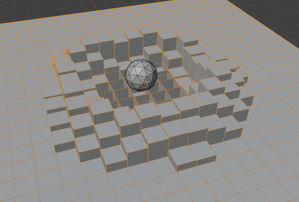
Move the driver object around the scene to change the extruded area of the grid. Adjust the values of the Map Range node to increase/decrease the effect. Add a Multiply Math node to increase the overall effect.

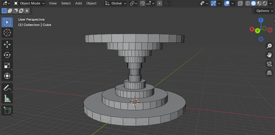
Result
Moving the driver object within the area of the grid changes the area that is extruded. By referencing the outside object, we can access all of its Attributes via Field nodes for use inside of the Node Group.
Bonus Challenge
Following the steps results in the extrusion only increasing or decreasing the height in one direction. Try to see if you can create a smoothed transition from one increase to a second increase. It should be possible using only the Field nodes like the Map Range and Compare nodes, along with some more Boolean Math. It should result in something that looks like this:
Outro
In this article, we covered:
Attributes
Fields
Instancing
These three concepts are key to really grasping the power of Geometry Nodes. In every article going forward we’ll be utilizing some, if not all of them to help us make powerful node setups.
Next Week
We’ll be diving into Simulation Zones, Repeat Zones, and Baking out node setups.
Supporter Content
If you are a paid subscriber, keep an eye out on Monday, January 20th for a How-To Guide on creating complex shapes and objects within Geometry Nodes. It will include more details, more pointed instructions, and more insights into Geometry Nodes.
Make sure to subscribe to ensure you get full access to that guide or feel free to use a complimentary free viewing to check out MipMap’s paid content before you become a Supporter.
If you enjoyed this tutorial, please like and sign up for a free subscription to MipMap! Or, if you didn’t enjoy then leave a comment to let me know what I can do better for the future. Either way, thank you for reading MipMap!
- Adam